Short Course on R Tools
Deep Learning in R
Classical Programming vs Machine Learning
- Deep learning is often presented as algorithms that “work like the brain”, that “think” or “understand”.
- AI: the effort to automate intellectual tasks normally performed by humans.
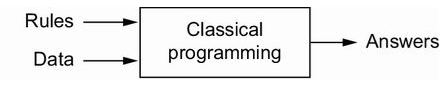
- ML: Could a computer surprise us? Rather than programmers crafting data-processing rules by hand, could a computer automatically learn these rules by looking at data?
![]()
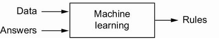
Artificial Intelligence
Machine learning
Deep learning
Classical Programming vs Machine Learning
- Deep learning is often presented as algorithms that “work like the brain”, that “think” or “understand”.
- AI: the effort to automate intellectual tasks normally performed by humans.
- ML: Could a computer surprise us? Rather than programmers crafting data-processing rules by hand, could a computer automatically learn these rules by looking at data?
![]()
Artificial Intelligence
Machine learning
Deep learning
Recipes of a Machine Learning Algorithm
- Input data points, e.g.
![]()
- If the task is speech recognition, these data points could be sound files
- If the task is image tagging, they could be picture files
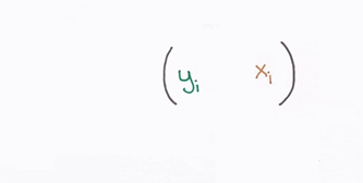
- Examples of the expected output
![]()
- In a speech-recognition task, these could be transcripts of sound files
- In an image task, expected outputs could tags such as “dog”, “cat”, and so on
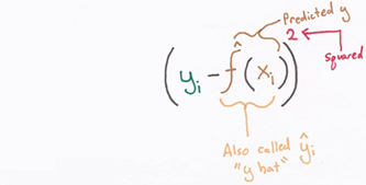
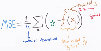
- A way to measure whether the algorithm is doing a good job
![]()
- This is needed to determine the distance between the output and its expected output.
- The measurement is used as a feedback signal to adjust the way the algorithm works.
![]()
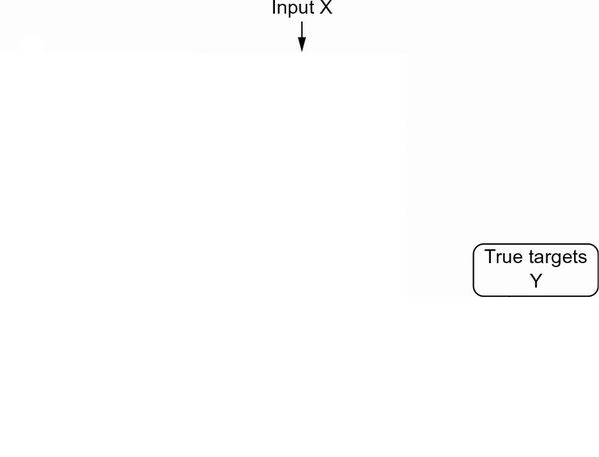
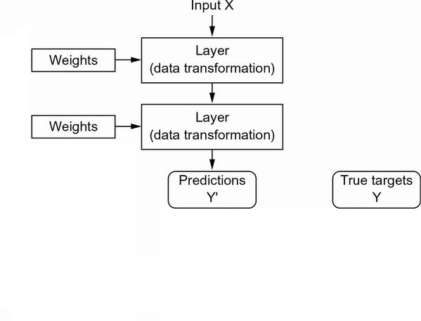
Anatomy of a Neural Network
The input data and corresponding targets
![]()
Layers, which are combined into a network (or model)
![]()
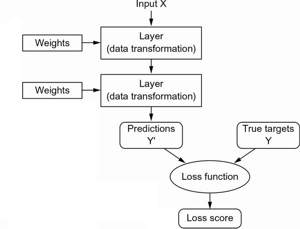
The loss function, which provides feedback for learning
![]()
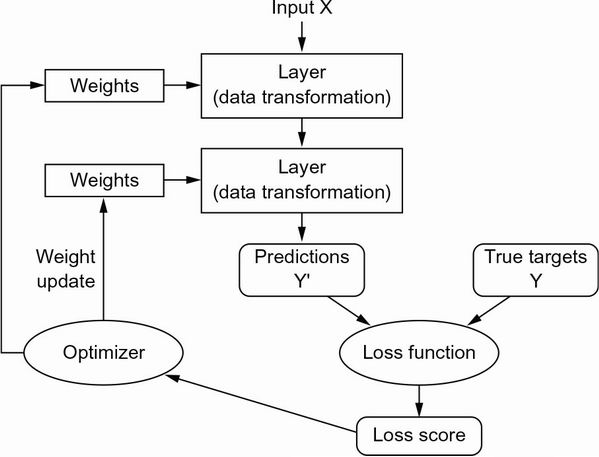
The optimizer, which determines how learning proceeds
![]()
LeNet-5: a pioneering 7-level CNN
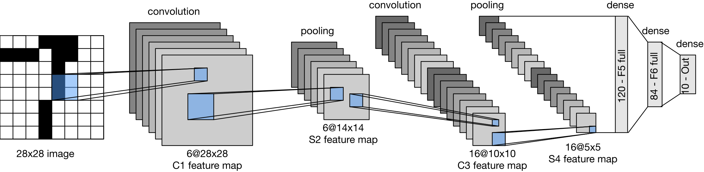
The first successful practical application of neural nets came in 1989 from Bell Labs, when Yann LeCun combined the earlier ideas of convolutional neural networks and backpropagation, and applied them to the problem of classifying handwritten digits.
The resulting network, dubbed LeNet, was used by the USPS in the 1990s to automate the reading of ZIP codes on mail envelopes.
LeNet-5 was applied by several banks to recognize hand-written numbers on checks digitized in 32x32 pixel images.
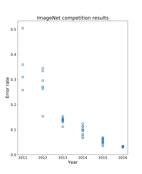
Why 30+ Years gap?

In 2011, Dan Ciresan from IDSIA (Switzerland) began to win academic image-classification competitions with GPU-trained deep neural networks
in 2012, a team led by Alex Krizhevsky and advised by Geoffrey Hinton was able to achieve a top-five accuracy of 83.6%–a significant breakthrough (in 2011 it was only 74.3%).
![]()
Three forces are driving advances in ML:
- Hardware
- Datasets and benchmarks
- Algorithmic advances
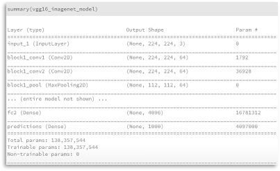
VGG16–CNN for Classification and Detection
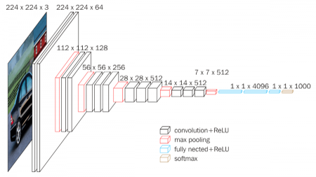
VGG16 is a convolutional neural network model proposed by K. Simonyan and A. Zisserman from the University of Oxford.
The model achieves 92.7% top-5 test accuracy in ImageNet. It was one of the famous model submitted to ILSVRC-2014.
It makes the improvement over AlexNet by replacing large kernel-sized filters (11 and 5 in the first and second convolutional layer, respectively) with multiple 3×3 kernel-sized filters one after another.
VGG16 was trained for weeks using NVIDIA Titan Black GPU’s.
![]()
Neural Network – Parameters - Activation Func.
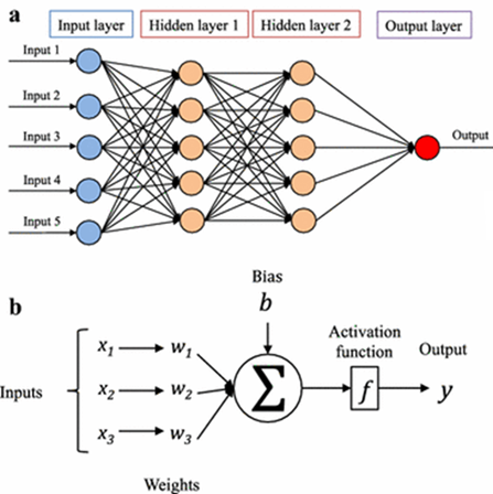
A Neural Network
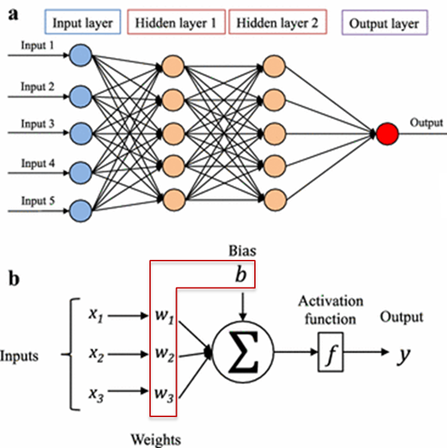
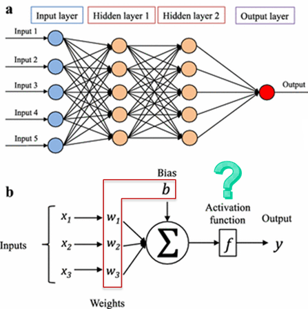
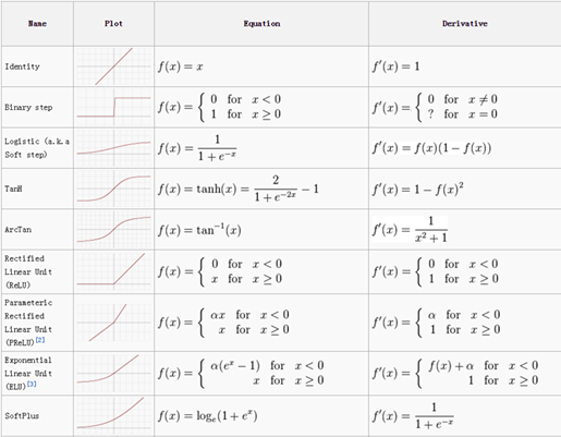
Activation Function
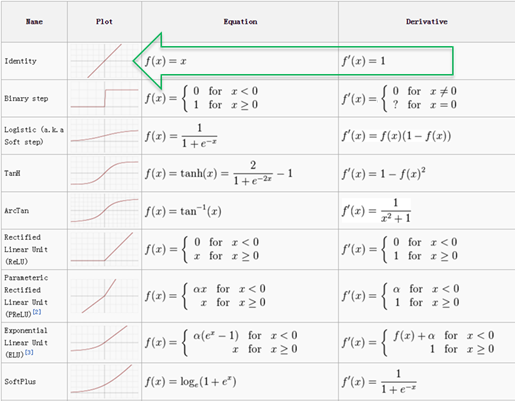
Linear Activation function
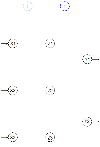
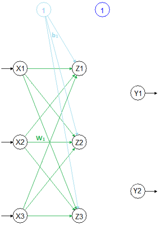
- \(Z=\color{green}{W_1}X+\color{lightblue}{b_1}\)
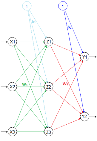
- \(Y=\color{red}{W_2}Z+\color{blue}{b_2}\)
- \(Y=\color{red}{W_2}\{\color{green}{W_1}X+\color{lightblue}{b_1}\}+\color{blue}{b_2}\)
- \(Y=\{\color{red}{W_2}\color{green}{W_1}\}X+\{\color{red}{W_2}\color{lightblue}{b_1}+\color{blue}{b_2}\}\)
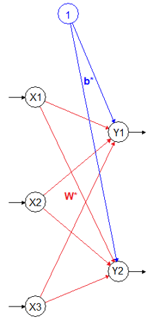
- \(Y=\color{red}{\mathbf{W}^*}X+\color{blue}{\mathbf{b}^*}\)
Hidden Layers Disappears
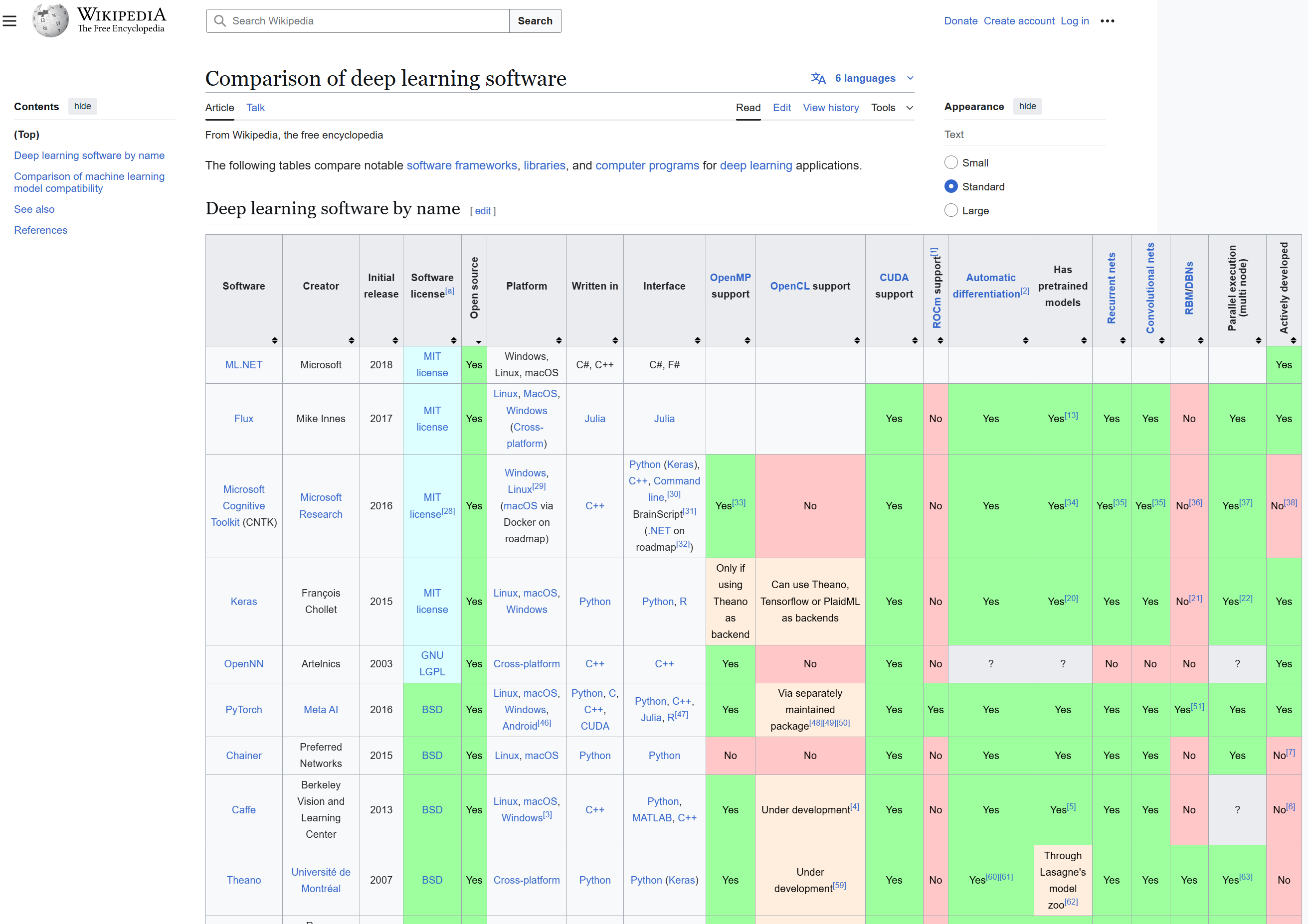
Deep learning software
What is TensorFlow?
- You define the graph in R
- Graph is compiled and optimized
- Graph is executed on devices
- Nodes represent computations
- Data (tensors) flows between them
Why TensorFlow in R?
- Hardware independent
- CPU (via Eigen and BLAS)
- GPU (via CUDA and cuDNN)
- TPU (Tensor Processing Unit)
- Supports automatic differentiation
- Distributed execution and large datasets
- Very general built-in optimization algorithms (SGD, Adam) that don’t require that all data is in RAM
- It can be deployed with a low-latency C++ runtime
- R has a lot to offer as an interface language for TensorFlow
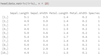
Real-world examples of data tensors
- 2D tensors
- Vector data—(samples, features)
![]()
![]()
- Vector data—(samples, features)

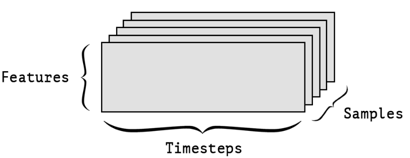
- 3D tensors
- Grayscale Images—(samples, height, width)
- Time-series data or sequence data—(samples, timesteps, features)

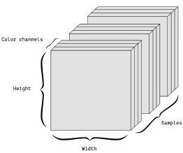
- 4D tensors
- Color Images—(samples, height, width, channels)

- 5D tensors
- Video—(samples, frames, height, width, channels)

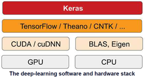
Why Keras?
- It allows the same code to run seamlessly on CPU or GPU.
- It has a user-friendly API that makes it easy to quickly prototype deep-learning models.

Installing Keras
- First, install the keras R package:
- To install both the core Keras library as well as the TensorFlow backend
- You need Python installed before installing TensorFlow
- Anaconda (Python distribution), a free and open-source software
- You can install TensorFlow with GPU support
- NVIDIA® drivers,
- CUDA Toolkit v9.0, and
- cuDNN v7.0
are needed: https://tensorflow.rstudio.com/tools/local_gpu.html
Developing a Deep NN with Keras
- Step 1 - Define your training data:
- input tensors and target tensors.
- Step 2 - Define a network of layers (or model)
- that maps your inputs to your targets.
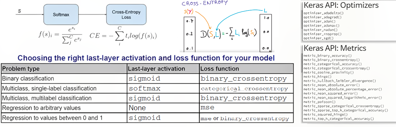
- Step 3 - Configure the learning process by choosing
- a loss function,
- an optimizer,
- and some metrics to monitor.
- Step 4 - Iterate on your training data by calling the
- fit() method of your model.
3. Multilayer Perceptrons (MLPs)
Keras: Step 1 – Data preprocessing
library(keras3)

# Load MNIST (Modified National Institute of Standards and Technology) images datasets
c(c(x_train, y_train), c(x_test, y_test)) %<-% dataset_mnist()

# Flatten images and transform RGB values into [0,1] range
x_train <- array_reshape(x_train, c(nrow(x_train), 784))
x_test <- array_reshape(x_test, c(nrow(x_test), 784))
x_train <- x_train / 255
x_test <- x_test / 255

# Convert class vectors to binary class matrices
y_train <- to_categorical(y_train, 10)
y_test <- to_categorical(y_test, 10)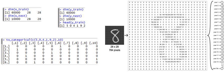
Keras: Step 2 – Model definition
model <- keras_model_sequential(input_shape = c(784))
model %>%
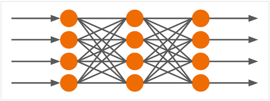
layer_dense(units = 256, activation = 'relu') %>%
layer_dropout(rate = 0.4) %>%
layer_dense(units = 128, activation = 'relu') %>%
layer_dropout(rate = 0.3) %>%
layer_dense(units = 10, activation = 'softmax')
summary(model)
># Model: "sequential"
># │ Layer (type) │ Output Shape │ Param # │
># ├-----------------------┼------------------┼---------┤
># │ dense_11 (Dense) │ (None, 256) │ 200,960 │
># │ dropout_3 (Dropout) │ (None, 256) │ 0 │
># │ dense_10 (Dense) │ (None, 128) │ 32,896 │
># │ dropout_2 (Dropout) │ (None, 128) │ 0 │
># │ dense_9 (Dense) │ (None, 10) │ 1,290 │
># └-----------------------┴------------------┴---------┘
># Total params: 235,146 (918.54 KB)
># Trainable params: 235,146 (918.54 KB)
># Non-trainable params: 0 (0.00 B)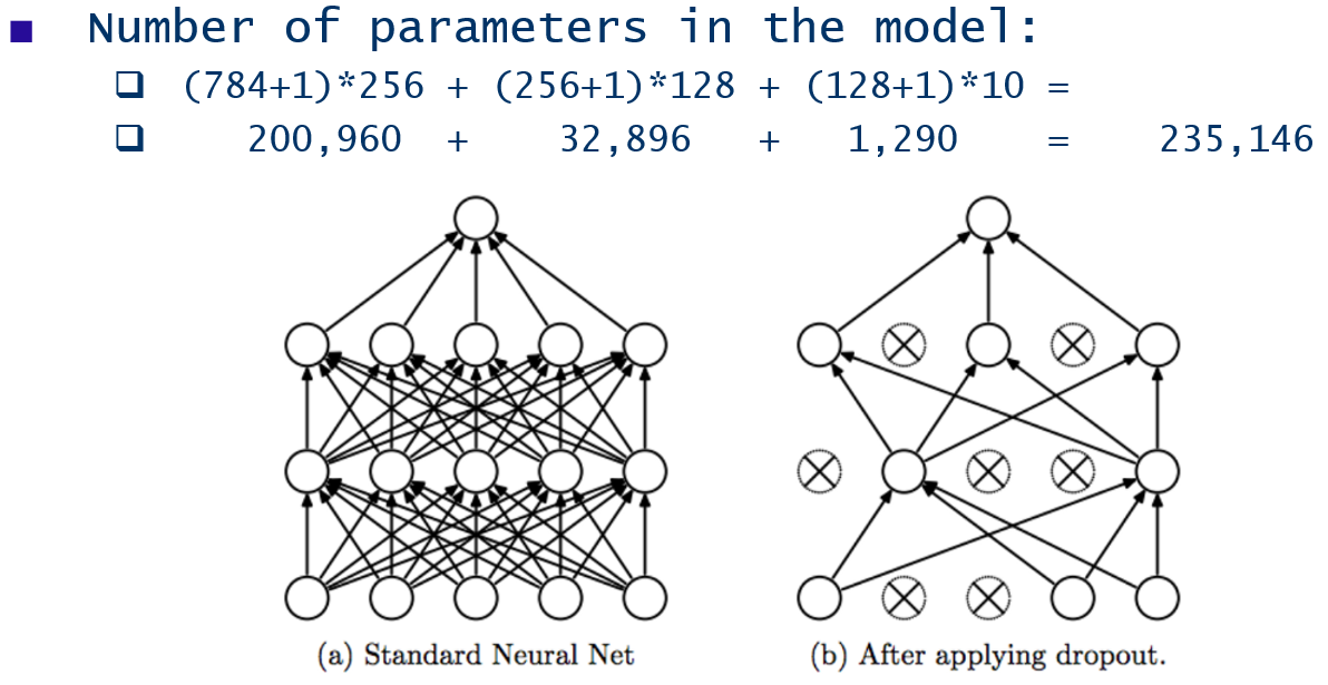
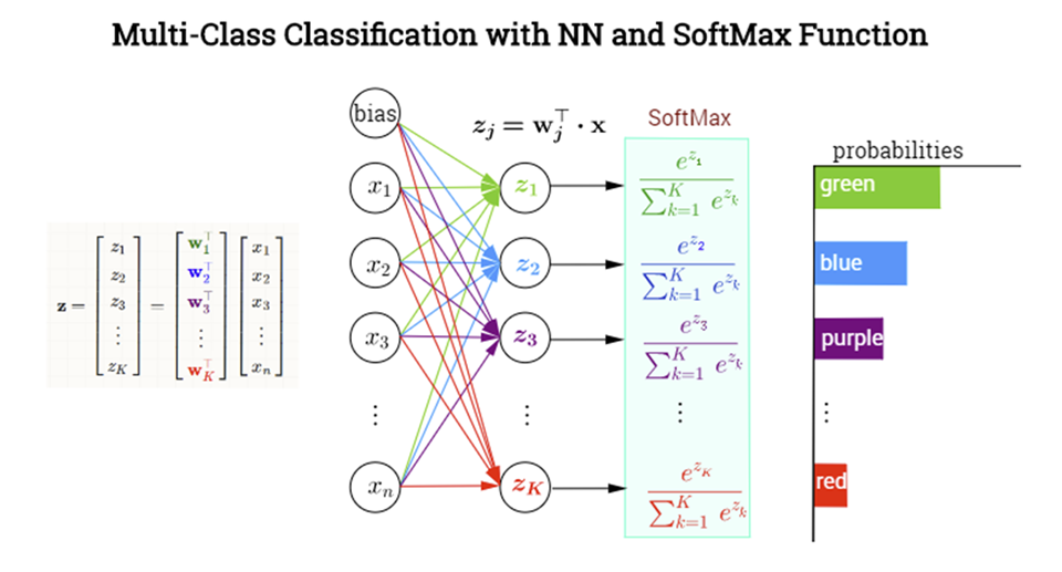
Multi-Class vs Multi-Label Classification
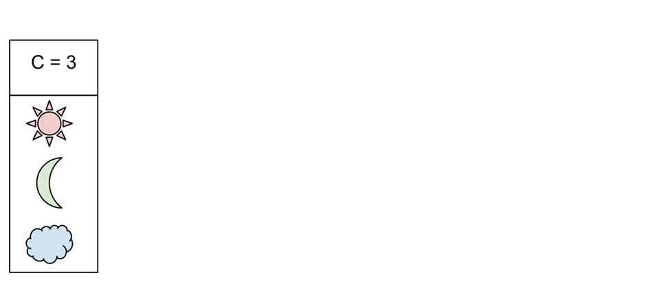
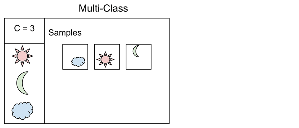
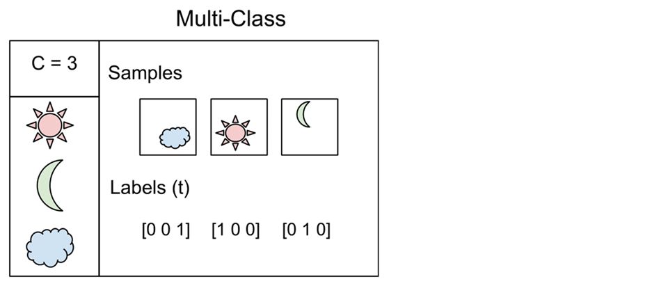
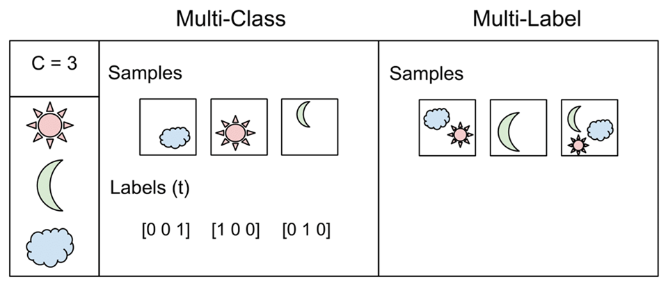
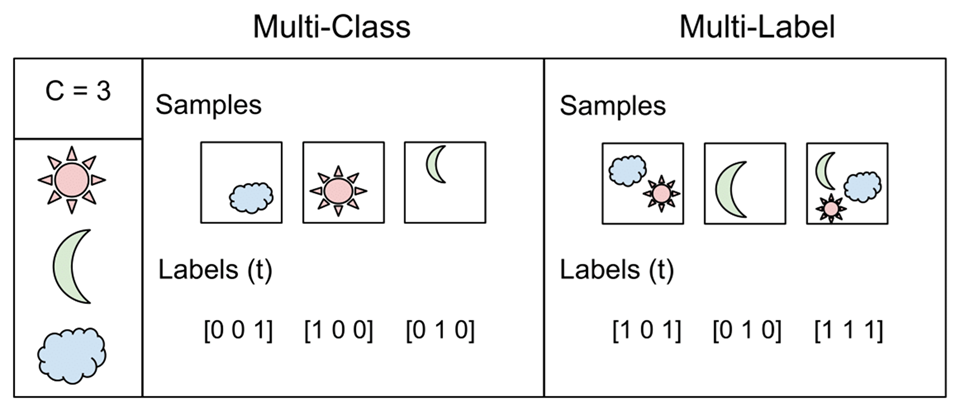
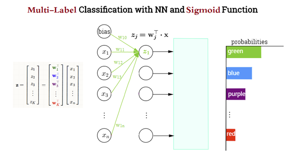
Multi-Class vs Multi-Label Classification (Cont.)

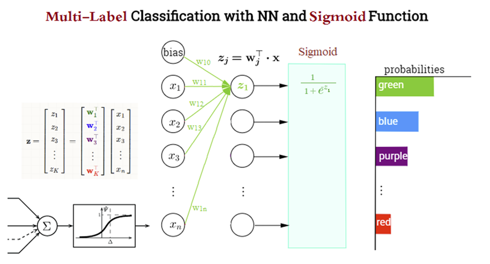
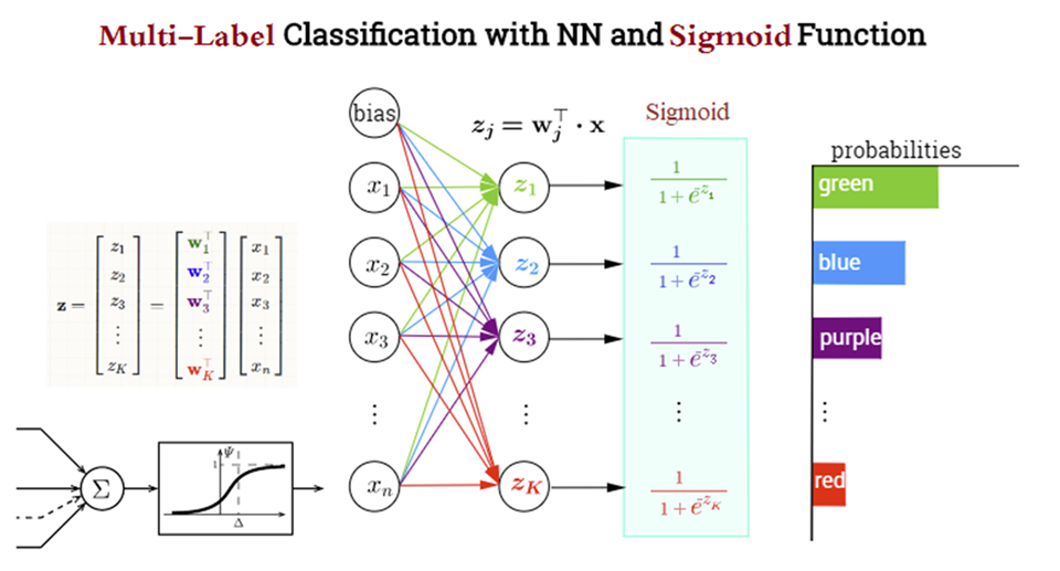
Multi-Class vs Multi-Label Classification (Cont.)
Keras: Step 3 – Compile Model
- Model compilation prepares the model for training by:
- Converting the layers into a TensorFlow graph
- Applying the specified loss function and optimizer
- Arranging for the collection of metrics during training
Keras: Step 4 – Model Training
- Use the
fit()to train the model for 10 epochs using batches of 128 images:- Feed 128 samples at a time to the model (batch_size = 128)
- Traverse the input dataset 10 times (epochs = 10)
- Hold out 20% of the data for validation (validation_split = 0.2)
Epoch 1/10
375/375 ━━━━━ 3s 5ms/step - accuracy: 0.7831 - loss: 0.6970 - val_accuracy: 0.9513 - val_loss: 0.1640
Epoch 2/10
375/375 ━━━━━ 1s 3ms/step - accuracy: 0.9371 - loss: 0.2123 - val_accuracy: 0.9628 - val_loss: 0.1249
Epoch 3/10
375/375 ━━━━━ 1s 3ms/step - accuracy: 0.9539 - loss: 0.1540 - val_accuracy: 0.9666 - val_loss: 0.1098
Epoch 4/10
375/375 ━━━━━ 1s 3ms/step - accuracy: 0.9612 - loss: 0.1301 - val_accuracy: 0.9743 - val_loss: 0.0865
Epoch 5/10
375/375 ━━━━━ 1s 3ms/step - accuracy: 0.9663 - loss: 0.1145 - val_accuracy: 0.9730 - val_loss: 0.0921
Epoch 6/10
375/375 ━━━━━ 1s 3ms/step - accuracy: 0.9688 - loss: 0.1020 - val_accuracy: 0.9736 - val_loss: 0.0923
Epoch 7/10
375/375 ━━━━━ 1s 3ms/step - accuracy: 0.9726 - loss: 0.0940 - val_accuracy: 0.9770 - val_loss: 0.0822
Epoch 8/10
375/375 ━━━━━ 1s 3ms/step - accuracy: 0.9742 - loss: 0.0875 - val_accuracy: 0.9770 - val_loss: 0.0815
Epoch 9/10
375/375 ━━━━━ 1s 3ms/step - accuracy: 0.9750 - loss: 0.0791 - val_accuracy: 0.9785 - val_loss: 0.0810
Epoch 10/10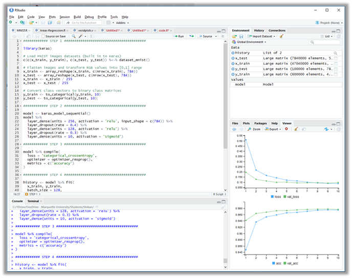
375/375 ━━━━━ 1s 3ms/step - accuracy: 0.9769 - loss: 0.0744 - val_accuracy: 0.9777 - val_loss: 0.0835Keras: Evaluation and prediction
plot(history)


model %>% predict(x_test[1:100,]) %>% apply(1, which.max)-1
># 4/4 ━━━━━━━━━━━━━━━━━━━━ 0s 957us/step
>#   [1] 7 2 1 0 4 1 4 9 6 9 0 6 9 0 1 5 9 7
>#  [19] 3 4 9 6 6 5 4 0 7 4 0 1 3 1 3 4 7 2
>#  [37] 7 1 2 1 1 7 4 2 3 5 1 2 4 4 6 3 5 5
>#  [55] 6 0 4 1 9 5 7 8 9 3 7 4 6 4 3 0 7 0
>#  [73] 2 9 1 7 3 2 9 7 7 6 2 7 8 4 7 3 6 1
>#  [91] 3 6 9 3 1 4 1 7 6 9

round(model %>% predict(x_test[1:9,]),5)
># 1/1 ━━━━━━━━━━━━━━━━━━━━ 0s 16ms/step
>#          [,1]    [,2]  [,3]  [,4]    [,5]    [,6]    [,7]    [,8]  [,9]   [,10]
>#  [1,] 0.00000 0.00000 0e+00 0.000 0.00000 0.00000 0.00000 1.00000 0e+00 0.00000
>#  [2,] 0.00000 0.00000 1e+00 0.000 0.00000 0.00000 0.00000 0.00000 0e+00 0.00000
>#  [3,] 0.00000 0.99983 1e-05 0.000 0.00001 0.00000 0.00000 0.00014 1e-05 0.00000
>#  [4,] 0.99986 0.00000 6e-05 0.000 0.00000 0.00000 0.00007 0.00000 0e+00 0.00000
>#  [5,] 0.00000 0.00000 0e+00 0.000 0.99995 0.00000 0.00000 0.00000 0e+00 0.00005
>#  [6,] 0.00000 0.99998 0e+00 0.000 0.00000 0.00000 0.00000 0.00002 0e+00 0.00000
>#  [7,] 0.00000 0.00000 0e+00 0.000 0.99984 0.00000 0.00000 0.00000 3e-05 0.00013
>#  [8,] 0.00000 0.00001 1e-05 0.002 0.00007 0.00007 0.00000 0.00044 4e-05 0.99737
>#  [9,] 0.00000 0.00000 0e+00 0.000 0.00000 0.30770 0.69230 0.00000 0e+00 0.00000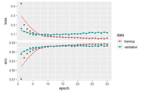
Keras Demo
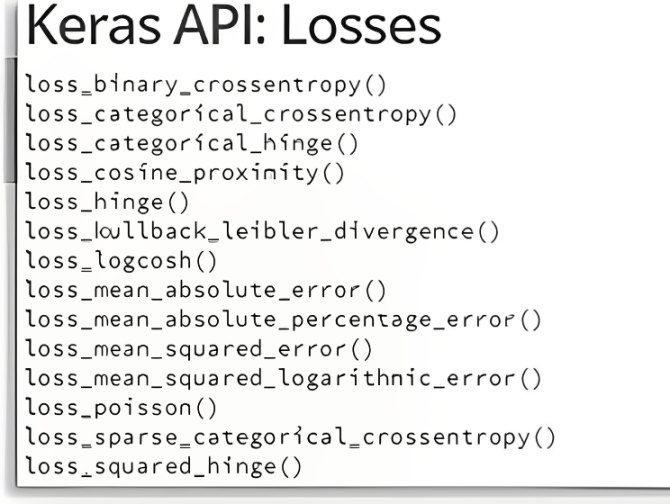
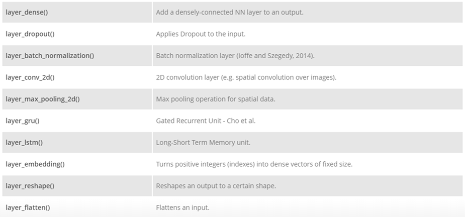
Keras API: Layers
- 90+ layers available (you can also create your own)
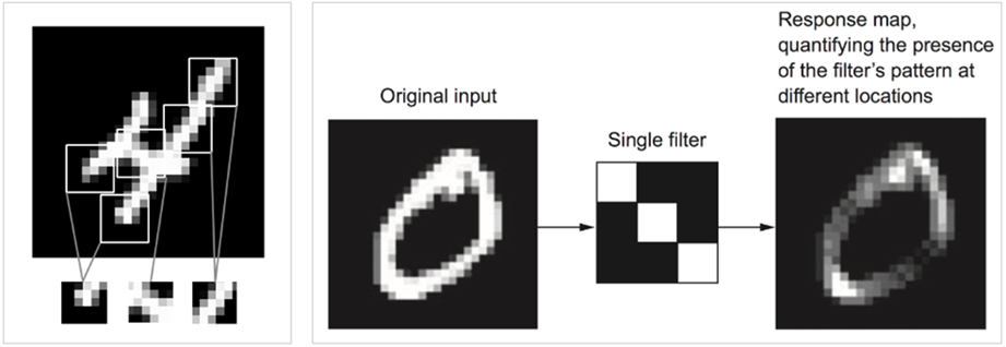
Convolutional Neural Networks (CNNs)
- Concepts: filters, pooling, feature maps
- Example:
cnn <- keras_model_sequential(input_shape=c(28,28,1)) %>%
  layer_conv_2d(filters=32, kernel_size=c(3,3), activation='relu') %>%
  layer_max_pooling_2d(pool_size=c(2,2)) %>%
  layer_conv_2d(filters=64, kernel_size=c(3,3), activation='relu') %>%
  layer_max_pooling_2d(pool_size=c(2,2)) %>%
  layer_flatten() %>%
  layer_dense(units=64, activation='relu') %>%
  layer_dense(units=10, activation='softmax')
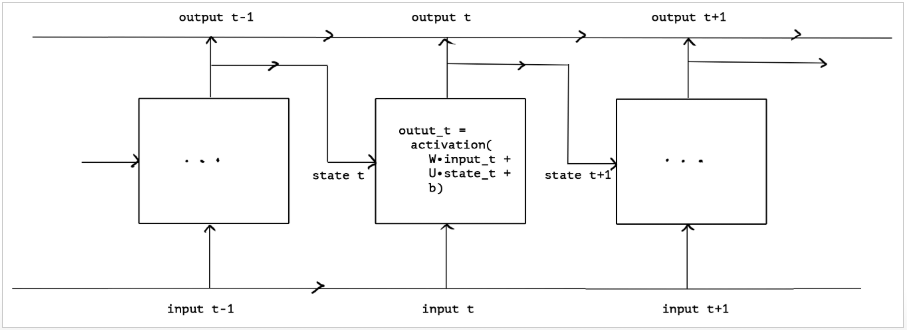
Recurrent Neural Networks & LSTM
- RNN basics: sequence data, time steps
- LSTM: handling long-term dependencies
- Use case: sentiment analysis, text generation
Embedding Layers
- Vectorization of text that reflects semantic relationships between words
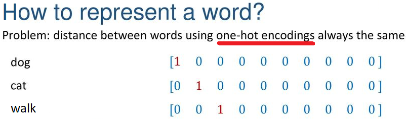
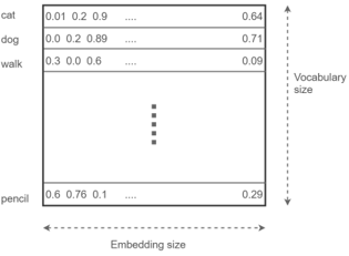
- How to use?
- Learn the embeddings jointly with the main task (e.g. classification); or
- Load pre-trained word embeddings (e.g. Word2vec, GloVe)
Autoencoders & Unsupervised Learning
- Architecture: encoder ⇄ bottleneck ⇄ decoder
- Applications: Dimension reduction, Denoising, Anomaly detection, Image segmentation, Neural inpainting

Hands-on Exercises
- Build and train a CNN on Fashion MNIST
- Implement an LSTM for
- Create an autoencoder for dimensionality reduction and visualize embeddings
![]()
Resources & Further Reading
- Book: Deep Learning with R by Francois Chollet & J.J. Allaire
![]()
- Deep Learning Book: https://www.deeplearningbook.org/
![]()
- Keras3 for R: https://keras3.posit.co/
- TensorFlow for R: https://tensorflow.rstudio.com/
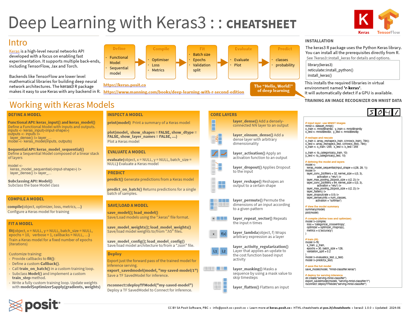
Keras for R cheatsheet
Q&A
Thank You
- Enjoy Deep Learning!
![]()